Title: Application of Multi-source Imagery in Landslide Detection — A Case Study of 2018 West Japan Flood
Overview
My Bachelor’s Thesis is mainly about detection of landslides triggered by extreme rainfalls using Sentinel-1 Synthetic Aperture Radar (SAR) imageries on Google Earth Engine (GEE) platform. In the thesis, I made a modification to the algorithm of Alexander L. Handwerger (2022) and enhanced the detection efficiency. Also, I made a comparison of the advantages and drawbacks between radar and optical imageries for their detection efficiency in rapid disaster response.
This blog is a translation of my thesis, which is originally written in Chinese and would be attached at the end of the blog.
Enormous thanks to Professor Xie Hu for her conscientious guidance throughout the completion of this thesis.
Abstract
Landslides often occur after events such as earthquakes and heavy rainfall, posing a significant threat to human life and property. After landslide occurrences, it is crucial to use imagery to detect and assess the distribution of landslides for effective disaster response. However, optical imagery is often inadequate for obtaining landslide information during rainfall-induced landslides due to cloud cover before and after the rainfall event. In such cases, the advantages of radar imagery become particularly prominent as it is not affected by cloud cover and can rapidly provide landslide information.
A study conducted by Handwerger et al. (2022) proposed a method for rapid landslide detection using synthetic aperture radar (SAR) data on the Google Earth Engine (GEE) platform. This paper further improved the method, enhancing its detection efficiency. Additionally, the study compared the advantages and disadvantages of radar imagery and optical imagery in the context of rapid landslide detection.
1 Research Background
1.1 2018 Western Japan Flood
From June 28 to July 8, 2018, Western Japan experienced intense rainfall, resulting in a significant number of mud floods and landslides. Nearly 200 people were killed in this incident, and more than 20,000 buildings were damaged. Hiroshima Prefecture was, in particular, severely affected. Figure 1-3 shows the false color composite images obtained from Sentinel-2 60 days before and after the event in the study area.
1.2 Area of Interest (AOI)
To maintain consistency and facilitate comparison, the Area of Interest (AOI) in this article remains consistent with the article by Handwerger et al., 2022. The AOI is a rectangle bounded by 34.28158°N in the north, 34.32469°N in the south, 132.66529°E in the west, and 132.71374°E in the east.
This AOI is covered by imageries from three Sentinel-1 paths, namely 83, 90 and 156. Among them, path 83 and 156 are ascending: 83 is to the east and 56 is to the west; whereas path 90 is descending.
2 Data and Platform
2.1 Sentinel-1 Radar Imageries
Sentinel-1 is an earth-observation mission by European Space Agency (ESA) comprising a constellation of two satellites, carrying C-band synthetic aperture radar (SAR) sensor with a wavelength of approximately 5.6 cm. The two satellites, Sentinel-1A and 1B, launched on April 3, 2014 and April 25, 2016 separately, each with a revisit cycle of 12 days, put together realize a revisit cycle of 6 days.
There are two common data products for Sentinel-1: SLC (Single Looking Complex) and GRD (Ground Range Detected). SLC is the original radar signal containing amplitude and phase, provides higher resolution and more information, but requires professional processing before it is ready to use.
GRD product is used in this thesis as there is no need of the phase data. Also, GRD is the only available Sentinel-1 data on Google Earth Engine. GRD data on GEE platform has been pre-processed through thermal noise removal, radiometric calibration and terrain correlation, thus is ready for consequent analysis. https://developers.google.com/earth-engine/datasets/catalog/COPERNICUS_S1_GRD
2.1.1 Observation Scenario
From the webpage of Sentinel-1 (https://sentinels.copernicus.eu/web/sentinel/copernicus/sentinel-1/acquisition-plans, https://sentinels.copernicus.eu/en/web/sentinel/copernicus/sentinel-1/acquisition-plans/observation-scenario-archive), for the area of Japan, all transmitted polarizations are vertical (V), but for the receive mode there are single or dual.
After the satellite was launched on April 3, 2014, the first public available imagery dates back on Cycle 29 during Sept. 30 to Oct. 12, 2014. Since then until Cycle 89 during Sept. 12 to 24, 2016, all acquisition modes are single vertical (VV), except for two cycles that are dual vertical (VV+VH): Cycle 65 during Nov. 29 to Dec. 11, 2015 and Cycle 79 during May 15 to 27, 2016.
From October 2016, observation on ascending paths are VV+VH, with a revisit cycle of 12 days; descending paths VV with a revisit cycle of 24 days.
From May 2017 (until October 2021, but in this thesis the last imagery dates back on May 18, 2020), both ascending and descending are dual polarization with revisit cycle of 12 days.
2.2.2 Side-looking of Radar Imageries
Unlike optical satellites which use nadir imaging, radar satellites employ side-looking imaging, resulting a larger imaging ranging. Because of this, for a specific study area, even if obtained from either ascending or descending paths, there could be multiple paths that cover this area. Since the Earth’s surface is not an ideal Lambertian reflector, there could be systematic difference of backscatter intensity due to the different look angles for different paths. Moreover, the same topography would also have different impacts on imaging for different paths. Therefore, it is inappropriate to make comparison among imageries acquired on different paths. In previous literatures, paths are only distinguished by ascending or descending, neglecting the difference of specific paths. In this thesis, I made a modification: calculation would only take place among imageries from the same paths, obtaining path-irrelevant results before combining.
2.2.3 Mechanism of Landslide Detection
In this thesis, the VH polarization is selected, which only exhibits relatively higher backscattering intensity when there is much volume scattering in the surface feature. Surface feature with high volume scattering includes dense vegetation and snow. Therefore, when landslide destroys vegetation and causes a bare ground, the intensity for VH polarization reduces, which could be detected from the intensity change in satellite imageries.
2.2 Sentinel-2 Optical Imageries
Sentinel-2 is another mission by ESA comprizing a constellation of two satellites, Sentinel-2A and 2B, launched on June 23, 2015 and March 7, 2017, separately. Each satellite has a revisit cycle of 10 days, used together makes a revisit cycle of 5 days for the constellation.
Sentinel-2 carries optical sensor called Multi-Spectral Imager (MSI), covering in total 13 bands from visible light to near-infrared. In this thesis, Band 4 (red, 10 m in spatial resolution) and Band 5 (NIR, 20 m in spatial resolution, resampled to 10 m to fit in the spatial resolution of Sentinel-1) were selected to calculate NDVI.
2.3 GSI-AJG Landslide Inventory
A report by Geospatial Information Authority of Japan (GSI) and The Association of Japanese Geographers (AJG) provides an inventory of the accurate location of landslides in this event, in which 7521 landslides were mapped with an average area of 2079 m2. The inventory is compiled from visual interpretation of high-resolution post-event aerial imageries, serves as the ground truth for this essay.
Click here to download the inventory.
2.4 NASADEM
Yet to be translated.
2.5 Google Earth Engine
Yet to be translated.
3 Data Processing and Algorithm
3.1 Generate Masks
Masks aim to filter out low-quality pixels and areas where landslides are unlikely to occur, enhancing the accuracy of detection. Masks used in the thesis include:
a) Quality Mask
Pixels with value lower than 30 dB are excluded, according to the manual of Sentinel-1.
b) Water Mask
Exclude water areas in the imageries. The water distribution information is stored in NASADEM as a band and could be accessed directly.
c) Slope Mask
Exclude flat areas with a threshold of 5° in this thesis. There is no readily available data for slope therefore it should be calculated from NASADEM.
d) Converture Mask
Exclude hilltop areas. In this thesis, positive curvature indicates terrain that is concave downward, while negative curvature indicates terrain that is convex upward. The threshold in this thesis is -0.005 m/m². Similarly, there is no readily available data for converture, and it should be calculated from NASADEM. A Gaussian filter has been applied to the DEM prior to calculation to eliminate high-frequency signals.
e) Valley Mask
As valley areas are relatively flat, they would be filtered out in the slope mask. However, unlike other plains, valleys are areas prone to be affected by landslides, thus they are re-included in this essay with a threshold of 0.003 m/m2.
3.2 Calculate SI value
The Susceptibility Index, denoted as SI, is the index proposed for landslide detection in this thesis. A higher SI value indicates a higher likelihood of being classified as a landslide. The calculation of SI value is as follows:
- Group imageries by paths.
- Choose a post-event imagery, and select every pre-event imageries from the same path, then subtract this post-event imagery from each pre-event imagery, resulting in a series of Iratio. As the unit of Sentinel-1 imageries is dB, the subtraction is the decibel value of the ratio of backscatter intensities of the two imageries:
- For each post-event imagery, calculate the average of Iratio, and assign a value of 1 to pixels with values greater than the 90th percentile, while setting other pixels to a value of 0. The outcome is denoted as individual SI.
- Calculate the average of the individual SI of all post-event imageries, resulting in the SI value.
3.3 Calculate AUC
The Area Under the Curve (AUC) is a commonly used indicator in machine learning and statistics for assessing the performance of binary classification models. AUC evaluates the overall quality of model predictions by calculating the area under the Receiver Operating Characteristic (ROC) curve. The ROC curve illustrates the relationship between the true positive rate (sensitivity) and the false positive rate (1 – specificity) at various thresholds. AUC values range from 0 to 1, with higher values indicating better classification performance. A value of 0.5 is equivalent as random guessing, while 1 signifies a perfect classifier.
Based on the ground truth data provided by GSI-AJG’s inventory, calculate the true positive rate and false positive rate for the SI values of individual pixels. Next, connect these data points in sequence to generate the ROC curve. The area beneath the curve is the AUC.
3.4 Calculate I_ad
The indicator proposed by Handwerger for landslide detection is denoted as I_ad (Intensity from ascending and descending imageries) in this thesis. Here is the brief summary of the algorithm:
- Separate all imageries by ascending and descending paths.
- Within each path group, further separate imageries into pre-event and post-event.
- Compute the median for each pixel within the four groups, resulting in four composite imageries.
- Subtract post-event imageries from corresponding pre-event imageries, resulting in I_ratio (Intensity ratio).
- Combine I_ratio from ascending and descending groups, resulting in I_ad.
4 Result
4.1 Masks Distribution Overview
Yet to be translated.
4.2 Generating Full Landslide Inventory
First, all available imageries were selected, considering the scenario of generating a full landslide inventory long after the event. To maintain consistency with Handwerger’s approach, the initial post-event imagery dates back to July 10, 2018, and the final post-event imagery to May 18, 2020. This results in a dataset comprising 131 imageries, spanning 678 days. For the pre-event period, all available images were selected, starting from May 3, 2015, until July 15, 2020, resulting in a dataset comprising 141 images, spanning 1169 days.
During the calculation process, imageries from different paths are not processed together, effectively grouping the imageries by their paths. With the exception of a relatively lower number of post-event imageries for path 156, the number of satellite imageries is approximately equal among the three paths.
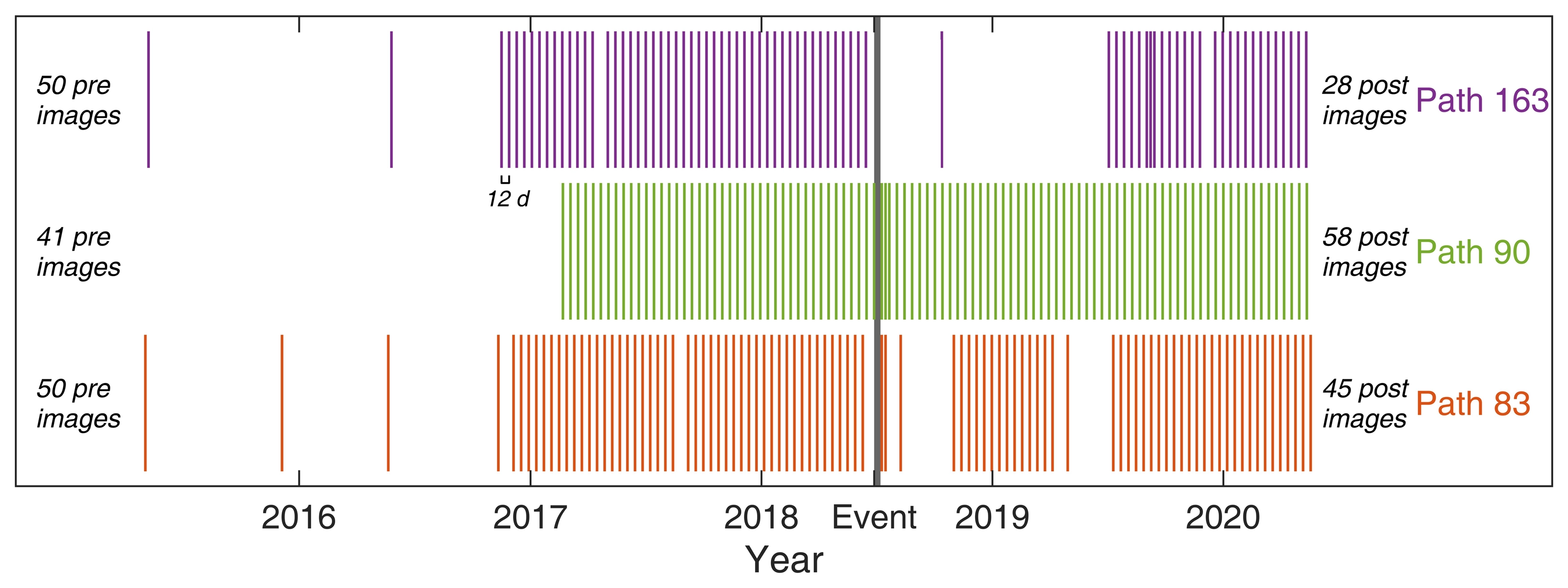
Figure 4-3 displays the ROC curve of SI values (in orange) calculated from imageries taken up to 678 days after the event, with a corresponding AUC value of 0.8709. As a reference, the ROC curve of I_ad from Handwerger’s approach (in blue) has an AUC value of 0.8335.
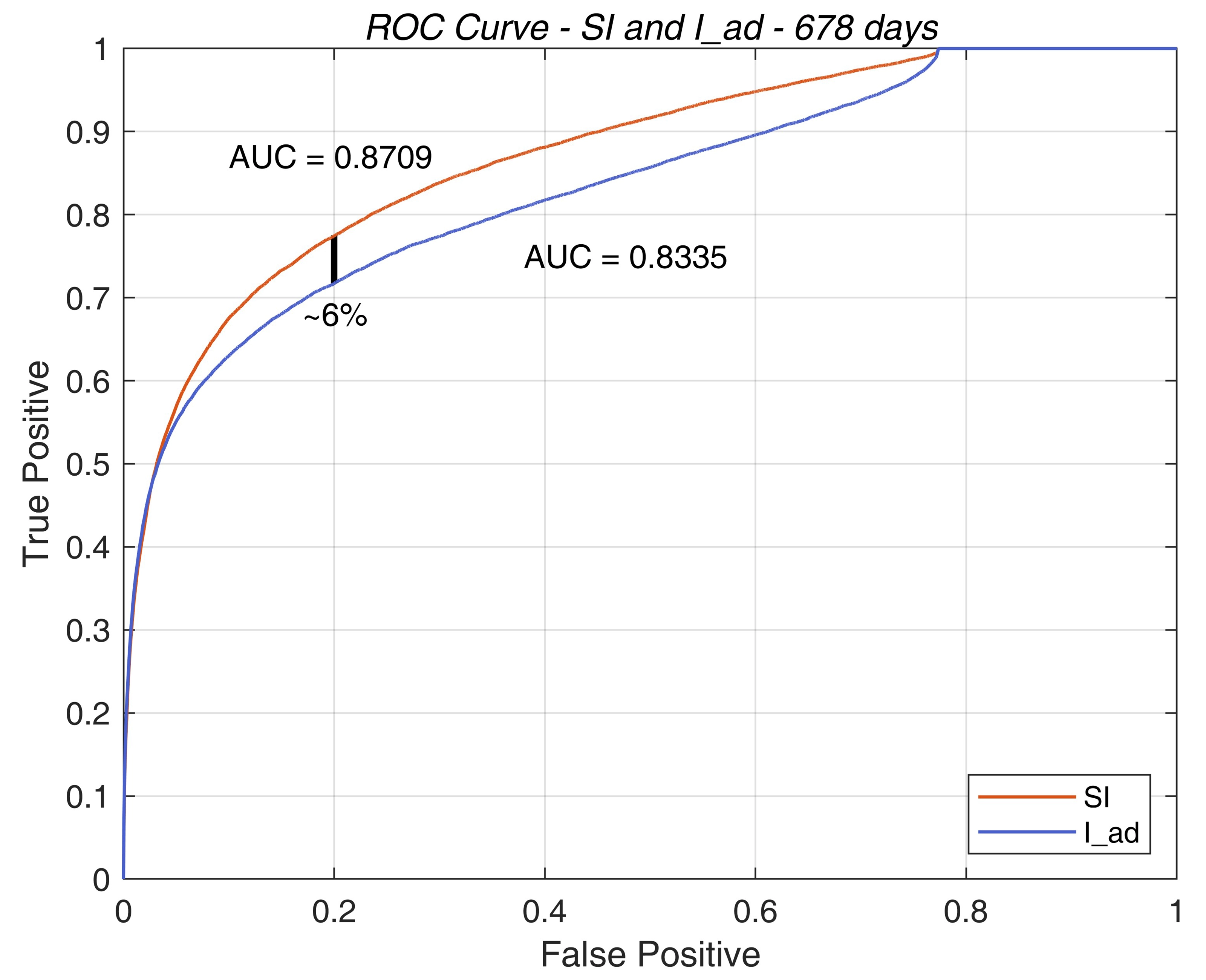
The SI value proposed in this thesis is calculated using the same dataset as I_ad in Handwerger’s approach, but with a significant improved AUC, highlighting the advantage of the new method.
4.3 AUC of Different Post-Event Days
Shorten the post-event imagery acquisition deadline to 4, 30, 90, 180, and 365 days to simulate scenarios of rapid response for disasters, and to explore the effects of the two methods at different time scales. The results are presented in the table below:
| Days After Event | Number of Images | AUC from SI | AUC from I_ad |
|---|---|---|---|
| 4 d | 2 images | 0.7073 | 0.6980 |
| 30 d | 6 images | 0.7734 | 0.7606 |
| 90 d | 12 images | 0.7867 | 0.7665 |
| 180 d | 26 images | 0.8018 | 0.7762 |
| 365 d | 52 images | 0.8436 | 0.8111 |
| 678 d | 131 images | 0.8709 | 0.8335 |
It is evident that SI outperforms I_ad, from the very first two imageries, to all available imageries until 678 days after the event. Additionally, it can be observed that AUC increases rapidly as the number of initial imageries accumulates; however, as the number of imageries reach a certain threshold, the increase of AUC begins to slow down.
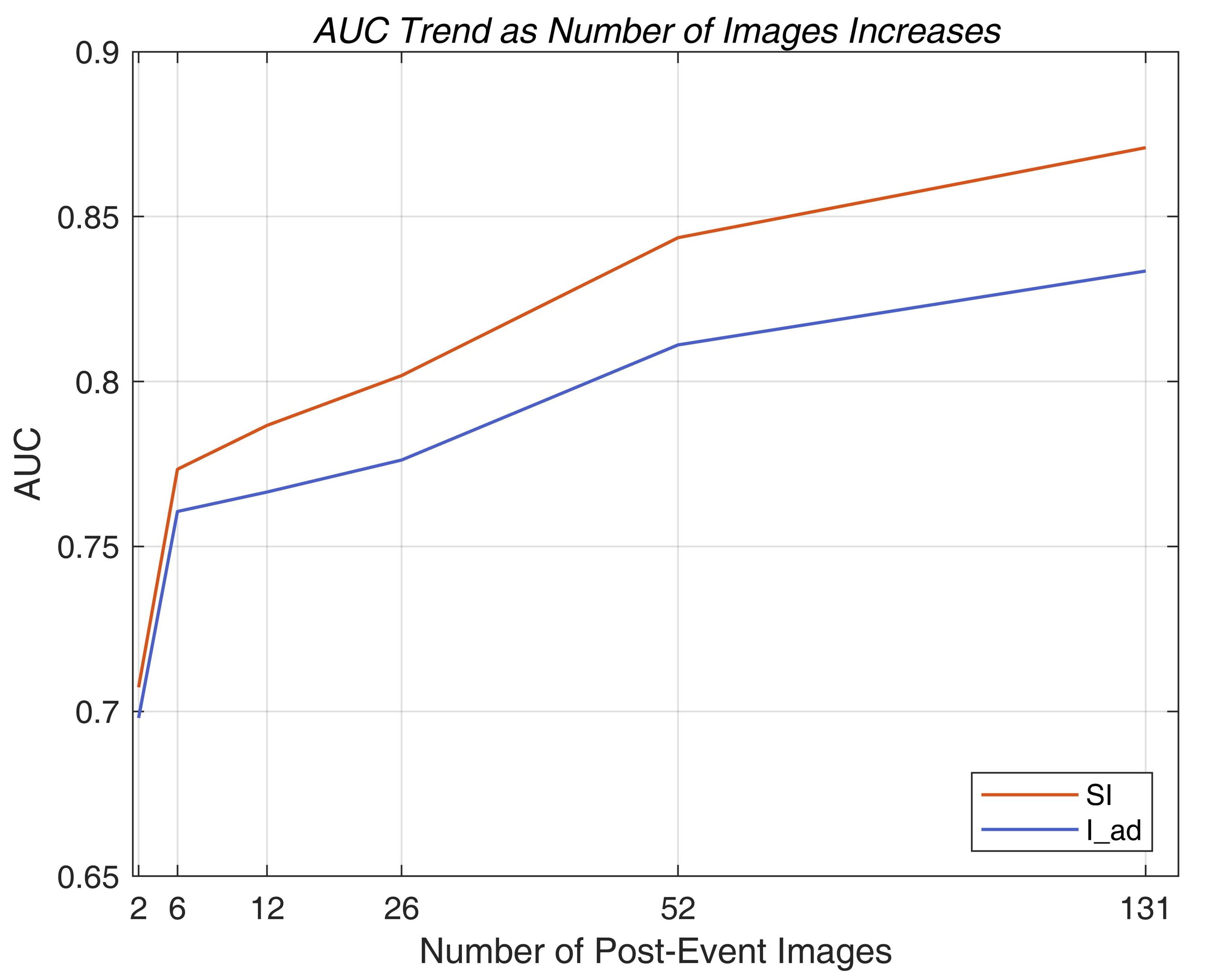
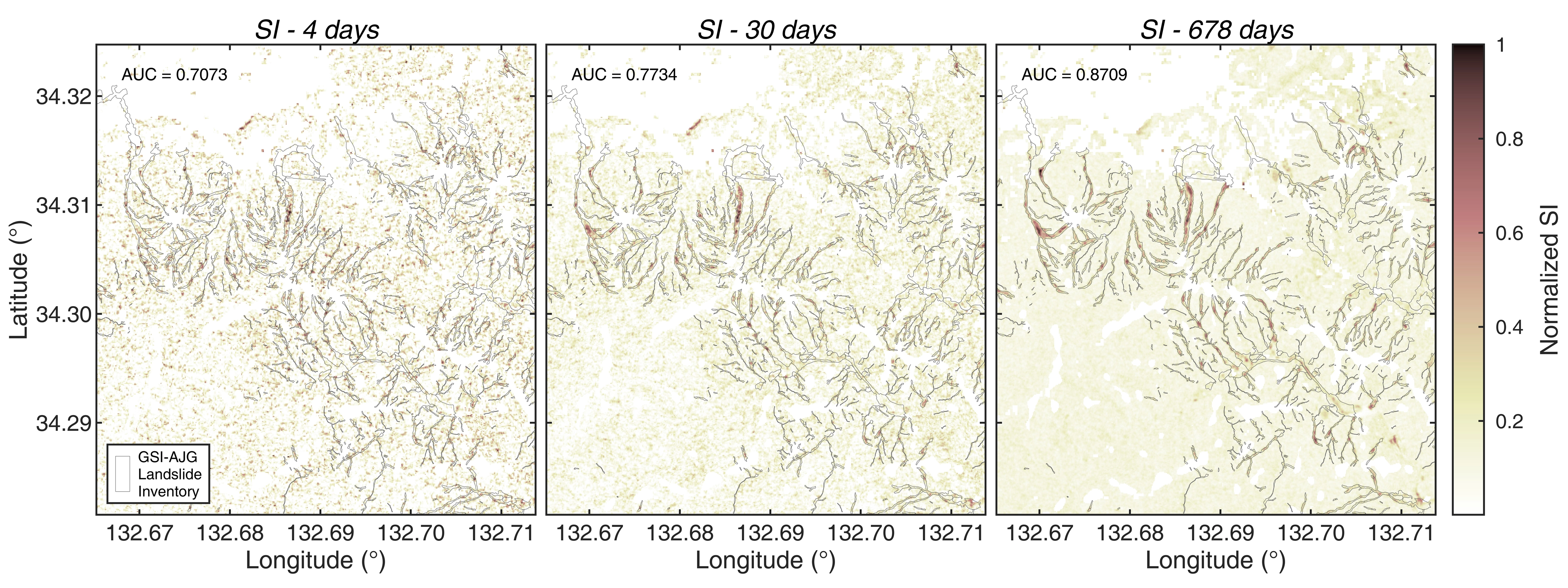
Figure 4-5 shows the spatial distribution of SI value from different numbers of post-event days. It can be observed that SI looks “messy” when the number of imageries is limited, and has a poor alignment with GSI-AJG inventory. When the number of imageries increases, the signal-to-noise ratio of SI increases correspondingly.
4.4 Comparison with Optical Imageries
Yet to be translated.
4.5 Simulation of Rapid Response
Figure 4-7 shows the AUC obtained from radar and optical imageries in limited time after the disaster has taken place. It can be observed that radar imageries yield an AUC of about 0.7 three days after the event. Though not ideal, it could still provide useful information of landslide distribution. Optical imageries also yield an AUC value four days after the event; however, it is worthless with the value of around 0.5, equivalent to random guessing. Only after nine days when there are available cloud-free optical imageries that they surpass radar imageries in terms of AUC. That is to say, for the period of 3-9 days after the event, radar imageries are capable of making a rough estimation of landslides, while optical imageries fall short.
5 Discussion
Yet to be translated.
Data Availability
The GEE codes in this thesis are available on Github. Please visit https://github.com/TsungRungWang/BachelorThesis.
You could also run the script directly on GEE: https://code.earthengine.google.com/682d9d9fd2809fc868762737e9d426c2. In line 88, codes from another script (getS1LIA) are called. Please refer to: https://code.earthengine.google.com/81cdb2dbc00fdc6107e28898fe11c365
Leave a Reply
You must be logged in to post a comment.